Python - Python Advanced - Numpy Tutorial

Numpy(Numerical Python) is a python package used for computational and processing of single dimension and multidimensional arrays.
Numpy is an extended module of python mainly written in c.
It provides a fast and efficient way to compute & handle a large number of data.
Numpy can only contain homogenous data.

Installation Of Numpy-

pip install numpy

Import NumPy, once installed-

import numpy as np

as - alias to create a short name for NumPy i.e np

Create NumPy array using-
The array object in NumPy is called ndarray.
We can create a NumPy ndarray object by using the array() function.

1] List
2] Tuple
3] Methods in NumPy using arange

1] List

a = [1,2,3,4,5,6]

array = np.array(a)
print(array , type(array))

Output-

[1 2 3 4 5 6] <class 'numpy.ndarray'>

2] Tuple

a = (1,2,3,4,5,6)

array = np.array(a)
print(array , type(array))

Output-

[1 2 3 4 5 6] <class 'numpy.ndarray'>

Dimensions in Arrays-
array.ndim to check dimension of array.
array.shape to check the shape of array.
array.size to check the size of array.

0-D Array
Also known as scalar. single value in the form of array known as 0-D array.

import numpy as np

arr = np.array(42)

print(arr, type(arr), arr.ndim)
print(arr.shape, arr.size)

Output-

42 <class 'numpy.ndarray'> 0
() 1

1-D Array
Also known as vector. collection of scalar is known as vector. Multiple 0-D array make a 1-D array(i.e single dimensional array).

import numpy as np

arr = np.array([23, 21, 19, 17, 15])

print(arr , type(arr), arr.ndim)
print(arr.shape, arr.size)

Output-

[23 21 19 17 15] <class 'numpy.ndarray'> 1
(5,) 5

2-D Array
Also known as matrix. collection of vector is known as matrix. Multiple 1-D array make a 2-D array(i.e two dimensional array).

import numpy as np

arr = np.array([[23, 21, 13], [19, 17, 15]])

print(arr , type(arr), arr.ndim)
print(arr.shape, arr.size)

Output-

[[23 21 13]
 [19 17 15]] <class 'numpy.ndarray'> 2
(2, 3) 6

3-D Array
Also known as multi dimensional array OR array of array. It is collection of matrix. Multiple 2-D array make a 3-D array(i.e two dimensional array).

import numpy as np

arr = np.array([[[23, 21, 13], [19, 17, 15]],[[1, 2, 3], [9, 7, 5]]])

print(arr , type(arr), arr.ndim)
print(arr.shape, arr.size)

Output-

[[[23 21 13]
  [19 17 15]]

 [[ 1  2  3]
  [ 9  7  5]]] <class 'numpy.ndarray'> 3
(2, 2, 3) 12

Create an array with high dimensional

import numpy as np

arr = np.array([14, 12, 30, 24], ndmin=4)

print(arr)
print('number of dimensions :', arr.ndim)

Output-

[[[[14 12 30 24]]]]
number of dimensions : 4

3] Create Array using Methods in numpy
i] arange - Creating array using range and step. And output will be in the form of 1-D array.

np.arange(1,20,2)

Output-

array([ 1,  3,  5,  7,  9, 11, 13, 15, 17, 19])

An array of odd number range from 1 to 20

ii] linspace - It will create an evenly spaced number in a specified interval.

np.linspace(1,10,16)

Output-

array([ 1. ,  1.6,  2.2,  2.8,  3.4,  4. ,  4.6,  5.2,  5.8,  6.4,  7. ,
        7.6,  8.2,  8.8,  9.4, 10. ])

iii] zeros - returns a new array of given shape and type, where the element's value as 0.

np.zeros(5)

Output-

array([0, 0, 0, 0, 0])

np.zeros((3,6))

Output-

array([[0., 0., 0., 0., 0., 0.],
       [0., 0., 0., 0., 0., 0.],
       [0., 0., 0., 0., 0., 0.]])

zeros like - Return an array of zeros with the same shape and type as a given array

a = [[1,2],[3,4],[5,6]]

array = np.array(a)
print(array , type(array))

Output-

[[1 2]
 [3 4]
 [5 6]] <class 'numpy.ndarray'>

np.zeros_like(array)

Output-

array([[0, 0],
       [0, 0],
       [0, 0]])

Default datatype of zeros() is a float.

iv] ones - returns a new array of given shape and type, where the element's value as 1.

np.ones(5)

Output-

array([1., 1., 1., 1., 1.])

ones like - Return an array of ones with the same shape and type as a given array

np.ones_like(array)

Output-

array([[1, 1],
       [1, 1],
       [1, 1]])

v] Identity matrix - eye
Identity matrix, also known as Unit matrix, is a "n ☓ n" square matrix with 1's on the main diagonal and 0's elsewhere.

np.eye(5)

Output-

array([[1., 0., 0., 0., 0.],
       [0., 1., 0., 0., 0.],
       [0., 0., 1., 0., 0.],
       [0., 0., 0., 1., 0.],
       [0., 0., 0., 0., 1.]])

To check all the function of numpy-
dir(numpy)
OR
dir(np) <-- with alias

Random Array-
It will create array of random element of a given dimension.

np.random.rand(2,3)

Output-

array([[0.05818802, 0.77241206, 0.49764276],
       [0.25382496, 0.58649652, 0.30227362]])

Reshaping the array
The numpy.reshape() function allows us to reshape an array in Python by changing dimension.

# Reshaping
# 1D (6) -> 2D(2x3, 3x2)
a = np.arange(6)
print(a)
print(a.reshape(6,1))
print(a.reshape(1,6))
print(a.reshape(2,3))
print(a.reshape(3,2))

Output-

[0 1 2 3 4 5]

[[0]
 [1]
 [2]
 [3]
 [4]
 [5]]

[[0 1 2 3 4 5]]

[[0 1 2]
 [3 4 5]]

[[0 1]
 [2 3]
 [4 5]]

print(a.reshape(3,-1))
print(a.reshape(2,3,-1))

Output-

[[0 1]
 [2 3]
 [4 5]]
[[[0]
  [1]
  [2]]

 [[3]
  [4]
  [5]]]

In above example it will automatically adjust unknown ddimension as per the known dimension.We can also create 3D array. We can only specify one unknown dimension, otherwise it will throw "ValueError: can only specify one unknown dimension".

Infer
Mostly used in machine learning or deep learning to create sample data.

array = np.arange(18).reshape(6,3)
array

Output-

array([[ 0,  1,  2],
       [ 3,  4,  5],
       [ 6,  7,  8],
       [ 9, 10, 11],
       [12, 13, 14],
       [15, 16, 17]])

Matrix Transpose-
Transpose of a matrix is the interchanging of rows and columns. It is denoted as X'. The element at ith row and jth column in X will be placed at jth row and ith column in X'. So if X is a 3x2 matrix, X' will be a 2x3 matrix.

matrix - i x j
Transpose matrix - j x i

array.T
array.T.shape

Output-

array([[ 0,  3,  6,  9, 12, 15],
       [ 1,  4,  7, 10, 13, 16],
       [ 2,  5,  8, 11, 14, 17]])
(3, 6)

Ravel or Flatten - To convert any dimensional array to one dimensional array.

array.flatten()

Output-

array([ 0,  1,  2,  3,  4,  5,  6,  7,  8,  9, 10, 11, 12, 13, 14, 15, 16,
       17])

array.ravel()

Output-

array([ 0,  1,  2,  3,  4,  5,  6,  7,  8,  9, 10, 11, 12, 13, 14, 15, 16,
       17])

Difference between ravel and flatten

Ravel-
return the reference of the original array
If you modify the ravel array, then original array will also change.
It is faster than flatten().

Flatten-
return the copy of the original array
If you modify the flattened array, then the original array will not be affected.
It is slower than flatten().

Basic Operation on Numpy Array

Arithmetic Operation on array is elementwise. (i.e no. of element should be the same)

Example-

a = np.array([10,20,30,40])
b = np.array([11,22,33,44])
print(a+b) #addition
print(a-b) #subtraction
print(a*b) #multiplication
print(a/b) #division
print(a%b) #modulus

Output-

[21 42 63 84]
[-1 -2 -3 -4]
[ 110  440  990 1760]
[0.90909091 0.90909091 0.90909091 0.90909091]
[10 20 30 40]

Comparison And Equality Operation

a = np.array([10,20,30,40])
b = np.array([20,11,30,50])
#Comparision Operator
print(a>b) #Greater Than
print(a<b) #Less Than
print(a>=b) #Greater Than or equal to
print(a<=b) #Less Than or equal to

#Equality Operator
print(a==b) #equal to
print(a!=b) #Not equal to

Output-

[False  True False False]
[ True False False  True]
[False  True  True False]
[ True False  True  True]
[False False  True False]
[ True  True False  True]

Matrix Multiplication
To multiply an m×n matrix by an n×p matrix, the m*n=n*p must be the same, and the result is an m×p matrix.
It is performed using dot()
A = n * m
B = m * p
C = A * B = n * p

Example-

A = np.array([[1,2,3] , [4,5,6]])
print(A,A.shape)
B = np.array([[1,4],[2,5] , [3,5]])
print(B,B.shape)

C = A.dot(B)
print(C,C.shape)

Output-

[[1 2 3]
 [4 5 6]] (2, 3)
[[1 4]
 [2 5]
 [3 5]] (3, 2)
[[14 29]
 [32 71]] (2, 2)

Unary Operation
To find the sum of array.

a = np.arange(24).reshape(4,6)
a

Output-

array([[ 0,  1,  2,  3,  4,  5],
       [ 6,  7,  8,  9, 10, 11],
       [12, 13, 14, 15, 16, 17],
       [18, 19, 20, 21, 22, 23]])

# sum
a.sum()

Output-

Axiswise

# give sum axiswise
"""
axis = 1 --> rowise
axis = 0 --> column wise
"""
print(a.sum(axis = 1))
print(a.sum(axis = 0))

Output-

[ 15  51  87 123]
[36 40 44 48 52 56]

# min & max

print(a.min())
print(a.max())

Output-

1
23

# min and max - row and column wise respectively

print(a.min(axis = 1))
print(a.min(axis = 0))
print(a.max(axis = 1))
print(a.max(axis = 0))

Output-

[ 0  6 12 18]
[0 1 2 3 4 5]
[ 5 11 17 23]
[18 19 20 21 22 23]

Universal FunctionArithmetic-

a = np.array([10,20,30,40])
b = np.array([3,4,7,4])

print(np.add(a,b))
print(np.subtract(a,b))
print(np.multiply(a,b))
print(np.divide(a,b))
print(np.mod(a,b))

Output-

[13 24 37 44]
[ 7 16 23 36]
[ 30  80 210 160]
[ 3.33333333  5.          4.28571429 10.        ]
[1 0 2 0]

Square root, square, trigonometry, and logarithm

print(np.sqrt(a))
print(np.square(b))
print(np.sin(a))
print(np.cos(a))
print(np.tan(a))
print(np.log(b))

Output-

[3.16227766 4.47213595 5.47722558 6.32455532]
[ 9 16 49 16]
[-0.54402111  0.91294525 -0.98803162  0.74511316]
[-0.83907153  0.40808206  0.15425145 -0.66693806]
[ 0.64836083  2.23716094 -6.4053312  -1.11721493]
[1.09861229 1.38629436 1.94591015 1.38629436]

Mean, Median & Mode

a = np.arange(24).reshape(6,4)
a

Output-

array([[ 0,  1,  2,  3],
       [ 4,  5,  6,  7],
       [ 8,  9, 10, 11],
       [12, 13, 14, 15],
       [16, 17, 18, 19],
       [20, 21, 22, 23]])

print(np.mean(a)) #OR print(a.mean())
print(np.median(a))

Output-

11.5
11.5

print(np.mean(a , axis = 0))
print(np.mean(a , axis = 1))

Output-

[10. 11. 12. 13.]
[ 1.5  5.5  9.5 13.5 17.5 21.5]

For mode-

from statistics import mode
a = (1,2,1,2,1,23,2,3,3,32,2)
mode(a)

Output-

Standard Deviation & Variance-

print(np.std(a))
print(np.var(a))

Output-

6.922186552431729
47.916666666666664

Indexing and slicing
Array indexing is the same as accessing an array element.
You can access an array element by referring to its index number. Index in numpy start from 0 to (length of array - 1).
Negative Indexing - From last, Indexing start from -1 to -(Length of array). therefore to access last element of array a, we can write a[-1].

Suppose we want to extract 8 from below array (1-D) then-

a = np.arange(1,10)
print(a)
print(a[7])

Output-

[1 2 3 4 5 6 7 8 9]
8

Suppose we want to extract last value from below array (1-D) then-

a = np.arange(1,10)
print(a)
print(a[-1])

Output-

[1 2 3 4 5 6 7 8 9]
9

Suppose we want to extract 18 from below array (2-D) then-

a = np.arange(28).reshape(7,4)
print(a)
print(a[4,2])

Output-

[[ 0  1  2  3]
 [ 4  5  6  7]
 [ 8  9 10 11]
 [12 13 14 15]
 [16 17 18 19]
 [20 21 22 23]
 [24 25 26 27]]
18

Slicing
Slicing in python means taking elements from one given index to another given index.

Syntax (for 1-D array)-

a[start:end]

We can also define step, for example-
a[start:end:step]

a = np.arange(1,10)

print(a)
print(a[2:8:2]))

Output-

[1 2 3 4 5 6 7 8 9]
[3 5 7]

Syntax (for 2-D array - Row and column)-

a[start_r:end_r,start_c:end_c]

We can also define step, for example-

a[start_r:end_r:step_r,start_c:end_c:step_c]

So on for any dimensional array

Example-

a = np.arange(28).reshape(7,4)
print(a)
print(a[1:4])

Output-

[[ 0  1  2  3]
 [ 4  5  6  7]
 [ 8  9 10 11]
 [12 13 14 15]
 [16 17 18 19]
 [20 21 22 23]
 [24 25 26 27]]
[[ 4  5  6  7]
 [ 8  9 10 11]
 [12 13 14 15]]

In the above program, rows 1,2, and 3 are extracted.

a = np.arange(28).reshape(7,4)
print(a)
print(a[1:4,1:3])

Output-

[[ 0  1  2  3]
 [ 4  5  6  7]
 [ 8  9 10 11]
 [12 13 14 15]
 [16 17 18 19]
 [20 21 22 23]
 [24 25 26 27]]
[[ 5  6]
 [ 9 10]
 [13 14]]

In the above program, row 1,2, and 3 are extracted, and column 1 and 2 is extracted.

a = np.arange(28).reshape(7,4)
print(a)
print(a[1:4,::2])

Output-

[[ 0  1  2  3]
 [ 4  5  6  7]
 [ 8  9 10 11]
 [12 13 14 15]
 [16 17 18 19]
 [20 21 22 23]
 [24 25 26 27]]
[[ 4  6]
 [ 8 10]
 [12 14]]

In the above program, row 1,2 and 3 are extracted, and columns with step 2( i.e columns 0, 3).

Iterating-
Iterating means going through elements one by one.

using for loop(1-D)-

a = np.array([1,2,3,4,5])
for i in a:
    print(i)

Output-

using for loop(2-D)-

a = np.arange(20).reshape(5,4)
a

Output-

array([[ 0,  1,  2,  3],
       [ 4,  5,  6,  7],
       [ 8,  9, 10, 11],
       [12, 13, 14, 15],
       [16, 17, 18, 19]])

for i in a:
    print(i)

Output-

[0 1 2 3]
[4 5 6 7]
[ 8  9 10 11]
[12 13 14 15]
[16 17 18 19]

for i in a:
    for j in i:
        print(j)

Output-

for i in a.flatten():
    print(i)

Output-

Splitting Of Array
We use np.split() for splitting arrays, we pass it the array we want to split and the number of splits.
Syntax-

np.split(array , int/list)

#int --> number of elements should be divisible by the int

Example-

array = np.arange(12)
array

Output-

array([ 0,  1,  2,  3,  4,  5,  6,  7,  8,  9, 10, 11])

np.split(array,6)

Output-

[array([0, 1]),
 array([2, 3]),
 array([4, 5]),
 array([6, 7]),
 array([8, 9]),
 array([10, 11])]

In the above program, array is split into 6 parts.

To access split array-

newarray = np.split(array,6)
print(newarray[2])
print(newarray[5])

Output-

[4 5]
[10 11]

Splitting the array using array-

array

Output-

array([ 0,  1,  2,  3,  4,  5,  6,  7,  8,  9, 10, 11])

"""
0-0
0-3 -> 0 2 4 6
4-6 -> 8 10 12
7-9 -> 14,16,18
10+ -> 20,22

"""
np.split(array , [0,4,7,10])

Output-

[array([], dtype=int32),
 array([0, 1, 2, 3]),
 array([4, 5, 6]),
 array([7, 8, 9]),
 array([10, 11])]

Splitting 2-D array

array = np.arange(24).reshape(4,6)
array

Output-

array([[ 0,  1,  2,  3,  4,  5],
       [ 6,  7,  8,  9, 10, 11],
       [12, 13, 14, 15, 16, 17],
       [18, 19, 20, 21, 22, 23]])

"""
axis - 1 - column wise
axis - 0 - row wise
"""

Splitting column into 3 part
np.split(array,3,axis = 1)

Output-

[array([[ 0,  1],
        [ 6,  7],
        [12, 13],
        [18, 19]]),
 array([[ 2,  3],
        [ 8,  9],
        [14, 15],
        [20, 21]]),
 array([[ 4,  5],
        [10, 11],
        [16, 17],
        [22, 23]])]

Splitting row into 2 part

np.split(array,2,axis = 0)

Output-

[array([[ 0,  1,  2,  3,  4,  5],
        [ 6,  7,  8,  9, 10, 11]]),
 array([[12, 13, 14, 15, 16, 17],
        [18, 19, 20, 21, 22, 23]])]

Vector Stacking / Concatenation

a = np.array([['saurabh','sachin','sulaj'] , ['Ramesh', 'akhil', 'ranjit']])
b = np.array([['atul','arjun'] , ['adi', 'ankitha']])
print(a)
print(b)

Output-

[['saurabh' 'sachin']
 ['Ramesh' 'akhil']]
[['atul' 'arjun']
 ['adi' 'ankitha']]

# rowise - number of columns of both the matrix should be the same
# columnwise - number of rows of both the matrix should be same

"""
axis 1 => columnwise
axis 0 --> rowise
"""

print(np.concatenate((a,b),axis = 0)) #Rowise 2 x 2 -> 4 x 2
print(np.concatenate((a,b),axis = 1)) #Columnwise 2 x 2 -> 2 x 4

Output-

[['saurabh' 'sachin']
 ['Ramesh' 'akhil']
 ['atul' 'arjun']
 ['adi' 'ankitha']]
[['saurabh' 'sachin' 'atul' 'arjun']
 ['Ramesh' 'akhil' 'adi' 'ankitha']]

If no. of columns or rows is not the same, then it will throw an error.

a = np.array([['saurabh','sachin','sulaj'] , ['Ramesh', 'akhil', 'ranjit']])
b = np.array([['atul','arjun'] , ['adi', 'ankitha']])
print(a)
print(b)

Output-

[['saurabh' 'sachin' 'sulaj']
 ['Ramesh' 'akhil' 'ranjit']]
[['atul' 'arjun']
 ['adi' 'ankitha']]

In the above array, no. of the column is not the same, a has three columns and b has 2 column-

print(np.concatenate((a,b),axis = 0)) #Rowise

Output-

---------------------------------------------------------------------------
ValueError                                Traceback (most recent call last)
Input In [12], in <cell line: 6>()
      1 """
      2 axis 1 => columnwise
      3 axis 0 --> rowise
      4 """
----> 6 print(np.concatenate((a,b),axis = 0))

File <__array_function__ internals>:180, in concatenate(*args, **kwargs)

ValueError: all the input array dimensions for the concatenation axis must match exactly,
 but along dimension 1, the array at index 0 has size 3 and the array at index 1 has size 2

So, it will throw ValueError. The same will happen if no. of rows is different.

Stacking
Syntax-

numpy.stack(arrays, axis=0, out=None)

Join a sequence of arrays along a new axis.

The axis parameter specifies the index of the new axis in the dimensions of the result. For example, if axis=0 it will be the first dimension, and if axis=-1 it will be the last dimension.

a = np.array([['saurabh','sachin'] , ['Ramesh', 'akhil']])
b = np.array([['atul','arjun'] , ['adi', 'ankitha']])
print(a)
print(b)

Output-

[['saurabh' 'sachin']
 ['Ramesh' 'akhil']]
[['atul' 'arjun']
 ['adi' 'ankitha']]

Using virtual stack instead of axis=0

np.vstack((a,b))

Output-

array([['saurabh', 'sachin'],
       ['Ramesh', 'akhil'],
       ['atul', 'arjun'],
       ['adi', 'ankitha']], dtype='<U7')

Using virtual stack instead of axis=1

np.hstack((a,b))

Output-

array([['saurabh', 'sachin', 'atul', 'arjun'],
       ['Ramesh', 'akhil', 'adi', 'ankitha']], dtype='<U7')

Copy & View

the main diff between a copy and a view of an array is that copy is a new array and view is just a view of original array

Deep Copy using copy()

arr = np.array([1,2,3,4,5])
print(id(arr))
x = arr.copy()
print(id(x))

x[0] = 42

print(arr)
print(x)

Output-

2519025518992
2519025519664
[1 2 3 4 5]
[42  2  3  4  5]

Shallow Copy using view()

arr = np.array([1,2,3,4,5])
print(id(arr))
x = arr.view()
print(id(x))

x[0] = 42

print(arr)
print(x)

Output-

2519025519472
2519025518992
[42  2  3  4  5]
[42  2  3  4  5]

Alias

arr = np.array([1,2,3,4,5])
print(id(arr))
x = arr
print(id(x))

x[0] = 42

print(arr)
print(x)

Output-

2519025520432
2519025520432
[42  2  3  4  5]
[42  2  3  4  5]

Using Skimage
Install it-

pip install scikit-image

Import-

import numpy
from skimage import data

Load image, check shape, size,dimension, and type of image

# load the image first
image = data.astronaut()
print(image.shape)
print(image.size)
print(image.ndim)
print(type(image))

Output-

(512, 512, 3)
786432
3
<class 'numpy.ndarray'>

image

Output-

array([[[154, 147, 151],
        [109, 103, 124],
        [ 63,  58, 102],
        ...,
        [127, 120, 115],
        [120, 117, 106],
        [125, 119, 110]],

       [[177, 171, 171],
        [144, 141, 143],
        [113, 114, 124],
        ...,
        [  0,   0,   0],
        [  1,   1,   1],
        [  0,   0,   0]]], dtype=uint8)

Import Matplotlib to use imshow() to show image-

import matplotlib.pyplot as plt

To show image-

plt.imshow(image)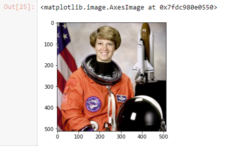

plt.imshow(image[0:220 , 100:350])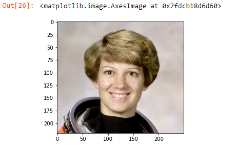

plt.imshow(image[0:300, 350:480])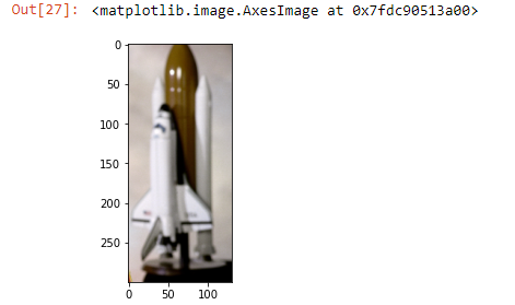

gray - (rows , columns , 1) # 1 for only one color

color- (row, column , 3) # 3 for RGB color

Python - Python Advanced - Numpy Tutorial

About Fresherbell

Important Links

Social Media